1
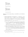
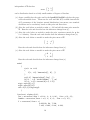
try to "see" from the contour plots for the log priors that priors i through iii are
ones of "independence" and the last two are not?
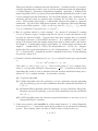
the product of Je¤reys improper priors, g ( ; ) = 12
a priori
N(0; 102 ) independent of 2 Inv- 2 (1; 102 )
a priori
N(0; 22 ) independent of 2 Inv- 2 (3; 22 )
the jointly conjugate prior discussed in Section 3.3 of the text, for
1; 0 = 1; 0 = 2
5. the jointly conjugate prior discussed in Section 3.3 of the text, for
10; 0 = 1; 0 = 2
1.
2.
3.
4.
0
= 0;
0
=
0
= 0;
0
=
> gsize<-101
> x<-c(4.90791,4.83425,5.19801,6.85308,4.07085,4.66076,
4.16201,5.49752,4.15438,3.72703)
> logL<- function (theta)
+ {
+ sum(log(dnorm(x,theta[1],theta[2])))
+ }
> mu<-3+seq(0,4,length=gsize)
> sigma<-.1+seq(0,2,length=gsize)
> theta<-expand.grid(mu,sigma)
> z<-apply(theta,1,logL)
> z<-matrix(z,gsize,gsize)
> plot(mu,sigma,type="n",main="LogLikelihood")
> contour(mu,sigma,z,levels=c(seq(-30,-10,1)))
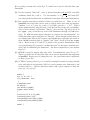
2. Consider a Bayes analysis of some bivariate normal data, under the complication that
not all of n = 10 data vectors are complete. In fact, suppose that observations are as
in the following table:
x1
3.683
7.189
5.014
4.946
3.495
4.065
4.222
-
x2
7.324
6.093
4.399
3.540
2.582
5.281
3.308
3.486
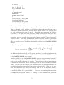
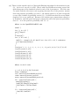
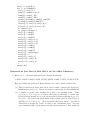
There is some OpenBUGS/WinBUGS code below that can be used to do an analysis
assuming that a priori the mean vector has
mean
0
0
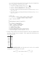
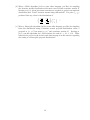
and covariance matrix
9
100 0
0 100