1
In the new formula, the Account specifier (A5) is correct but the Period specifier is now cell D3 — which is blank
and obviously not correct. In fact, the Company (A2), Year (B2), and Type (C2) are also incorrect now. To copy this
formula correctly, we will have to ensure that Excel does not adjust the cell references when we copy the formula.
This is called an Absolute reference and is accomplished by placing a dollar sign ($) before the parts of the reference
that do not change. For more information see the Excel Help Index.
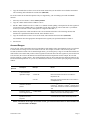
1.
Click on cell D4, and in the formula bar (located at the top of the spreadsheet, above the column names) move
your cursor to the Account reference (A4).
2.
Press ). Each time you press F4, Excel toggles through the combinations: absolute column and absolute row
($A$4), relative column and absolute row (A$4), absolute column and relative row ($A4), and relative column
and relative row (A4). We will want the Account reference to change as we copy down rows (relative, no $), but
not across columns (absolute, $). Press ) until the Account reference is $A4. You can also add the $ symbol
with the keyboard.
3.
We will not want the Period reference to change as we copy it down rows, but we will across columns (relative
column and absolute row). Make the Period reference D$2.
4.
The Company, Year, and Type cell references should not change when we copy the formula down or across the
report, so make both the column and row references absolute ($A$1).
5.
Press (QWHU.
The formula should now be: =GL($A4, D$2, $A$1, $B$1, $C$1) and is ready to be copied down all of the account
numbers.
$XWR)LOO
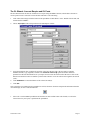
1.
Click on the cell in which the first GL formula is currently specified (D4). You will see a fill handle which is
located at the bottom right of the cell when it is selected. Move your mouse over the fill handle, and your pointer
will become a crosshair.
2.
Double click the fill handle. The formula will now copy down all rows that have a value in Column C. If there is
no value in Column C, or if your version of Excel does not support this feature, simply drag the formula down by
clicking and holding the left mouse button over the fill handle and dragging the formula until the last row with an
account number is selected.
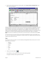
3.
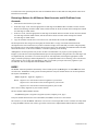
Click on any cell in your spreadsheet. You will notice that all of the cells have the same value as cell D4. This is
because the sheet is set for manual calculation. Press ) to calculate the workbook, and the values from your GL
will populate the report.
Because the Period specifier (cell D2) is currently the word "Month," the values returned are for the current (usually
open) period.
3DJH
$4XLFN7RXURI)