1
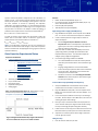
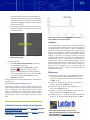
injection continuously delivers sample at the cross intersection, as shown in Figure 1. The injection plug size depends on the time and velocity of the injection. The advantage of this approach is the user has more variables to control for optimizing the separation downstream. The biggest drawback is an increased electrophoretic bias of the sample plug that is loaded. Figure 2 is a diagram of the chip channels and reservoirs. The sample is loaded by applying a 1 potential to the sample reservoir such that the relative fields are : Solutions Buffer: 10 mM Phosphate Buffer at pH ~7.2 Fluorenscent Sample: 10 mM Phosphate buffer (at pH ~7.2) with 1 mM sodium fluorescein Deionized (DI) water (18 MΩ) 100 mM potassium hydroxide (KOH) ESample ≤ E SampleWaste or EBuffer ≥ EBufferWaste. 1. To make an injection of the sample onto the analysis column, the electric field at the buffer reservoir is lowered or raised at the 1 sample reservoir such that the situation is reversed as in : 2. High-Voltage Power Supply (HVS448) Setup ESample ≥ E SampleWaste or EBuffer ≤ EBufferWaste. GOAL: The student/new practitioner will use this experiment to determine the best electric field strengths, flow rates and injection times to maximize their sample/reagent loading, signal-to-noise and separation efficiency. Gated Injection Experimental Setup Equipment and Materials LabSmith SVM340 Synchronized Video Microscope with uScope™ software o SVM340 Black and White Camera Module o Blue Illuminator o 10X DIN 0.25 Objective o 515 nm Long-pass Filter LabSmith HVS448 6000D High Voltage Sequencer with Sequence™ software o Platinum electrodes (4) o Micro-Clip connectors o High Voltage Cables 10-100 µL pipette with 100 µL pipette tips 0.2 µm solution filter Particle-free wipes Disposable nitrile gloves Safety goggles Glass cross-channel nanochip (Figure 2): 250 nm deep x 7.5 µm wide channels ( Dolomite chip, http://www.dolomitemicrofluidics.com/en/design/custom-devices ). 3. Inverted Microscope (SVM340) and Chip Setup 1. 2. 3. 4. 5. 6. Figure 2. Diagram of Microfluidic chip. Length of the channel W to E is 35 mm±0.30 mm; N to S is 10 mm ± 0.30mm Plug HVS448 into wall power and to computer via the RS232 port. Turn on the unit and launch the Sequence™ software. Create a new Sequence file using the steps in Table 1 for Sequence Steps A-F. a. See the Using the Sequence Wizards to Create a Sequence File section of the Sequence™ Users Manual (pp 13-17) for instruction on making a Simple Sequence Wizard and Running a Sequence. Note: The values in Table 1 were developed for use with a specific chip geometry and buffer pH as described in the Experimental Set-Up section. You will need to adjust the voltages if using a different configuration. Connect the high-voltage cables to the HVS448. a. Turn off the HVS448 and remove the interlock (50 ohm terminator) from the back of the unit to disable the high voltage. b. Plug high voltage cables A-D in channels HVA-HVD. c. Install a microclip and platinum electrode on the labeled end of each cable. Alternatively, press the electrode directly into the end of the cable. d. Follow the instructions in the Grounding the HVS4448 Channels section of the Sequence™ User’s Manual (pps. 11-12) to ground the unit. Setup the SVM340 with a black & white camera module installed with a 515 nm filter and a blue illuminator. Plug the SVM340 into wall power, into the computer via the RS232 port, and to the video capture card via USB port. Turn on the unit. Launch the uScope™ software and ensure you are viewing a live video. See the uScope™ User’s Manual for instructions on selecting the proper video settings. Place your chip on the stainless steel microscope plate and secure. Double-stick tape or magnets work well for holding the chip on the stage (the plate is magnetic stainless). Install reservoirs on the chip ports to allow the channels to be filled with fluid and provide a place to insert the electrodes. Adjust the X-Y and focus position of the stage to locate the channel region of interest. Filling the Chip 1. Filter all solutions with a 0.2 µm filter.