1
Defining Model Structures
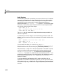
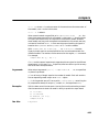
Polynomial Black-Box Models: The idpoly Model
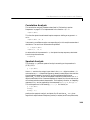
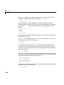
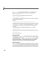
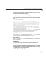
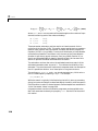
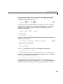
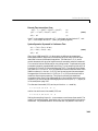
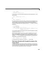
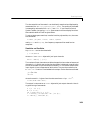
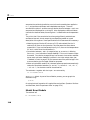
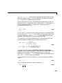
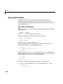
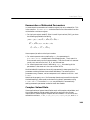
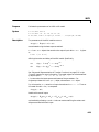
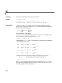
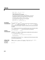
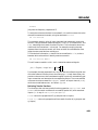
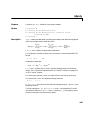
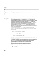
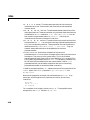
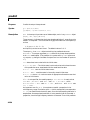
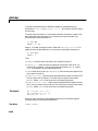
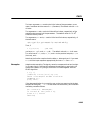
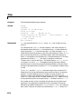
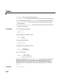
The general input-output form (3-19)
B(q)
C(q)
A ( q ) y ( t ) = ------------- u ( t – nk ) + ------------- e ( t )
F(q)
D(q)
(3-43)
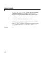
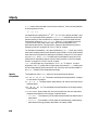
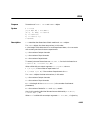
is defined by the five polynomials A(q), B(q), C(q), D(q), and F(q). These are
represented in the standard MATLAB format for polynomials. Polynomial
coefficients are stored as row vectors ordered by descending powers. For
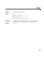
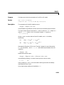
example, the polynomial
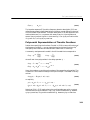
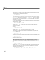
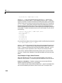
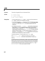
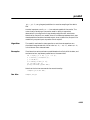
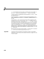
A ( q ) = 1 + a1 q
–1
+ a2 q
–2
+ … + an q
–n
is represented as
A = [1 a1 a2 ...
an]
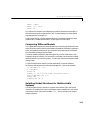
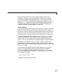
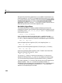
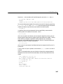
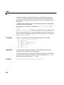
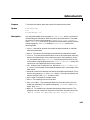
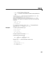
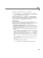
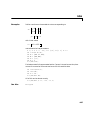
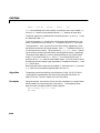
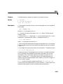
Delays in the system are indicated by leading zeros in the B ( q ) polynomial. For
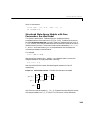
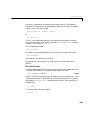
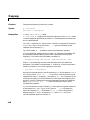
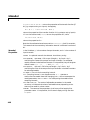
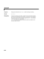
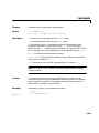
example, the ARX model
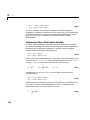
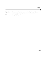
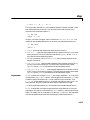
y ( t ) – 1.5 y ( t – 1 ) + 0.7 y ( t – 2 ) = 2.5u ( t – 2 ) + 0.9u ( t – 3 )
(3-44)
is represented by the polynomials
A = [1 -1.5 0.7]
B = [0 0 2.5 0.9]
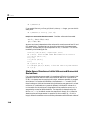
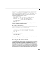
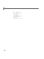
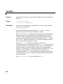
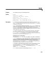
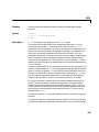
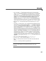
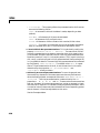
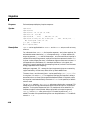
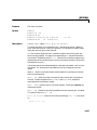
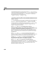
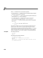
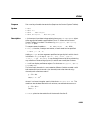
The idpoly representation of (3-43) is now created by the command
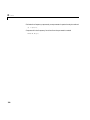
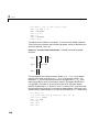
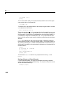
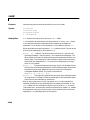
m = idpoly(A,B,C,D,F,lam,T)
lam is here the variance of the white noise source e ( t ) and T is the sampling
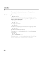
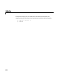
interval. Trailing arguments can be omitted for default values. The system
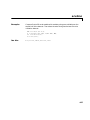
(3-44) can for example be represented by
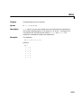
m = idpoly([1 -1.5 0.7],[0 0 2.5 0.9])
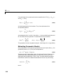
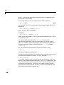
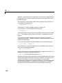
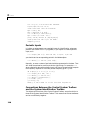
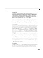
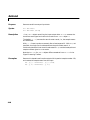
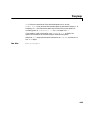
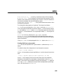
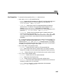
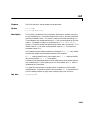
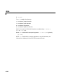
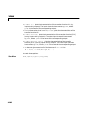
In the multi-input case (3-41) B and F are matrices, whose row number k
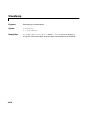
corresponds to the k-th input. The command idpoly can also be used to define
time-continuous systems. See Chapter 4, “Command Reference” for details.
3-37