1
Multicolumnand2Dlookup
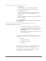
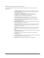
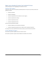
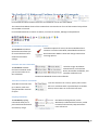
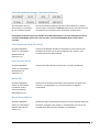
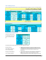
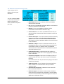
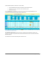
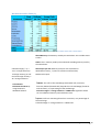
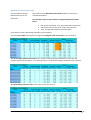
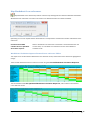
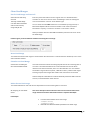
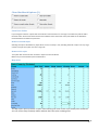
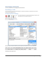
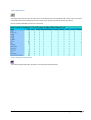
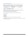
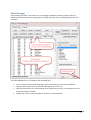
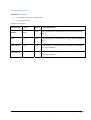
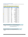
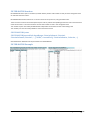
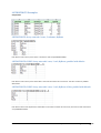
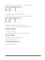
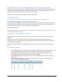
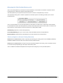
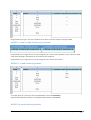
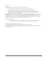
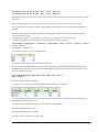
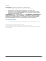
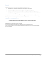
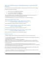
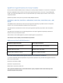
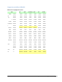
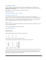
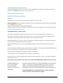
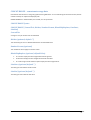
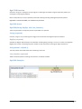
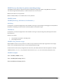
This example looks for a row with “superphone” in the “product” column and “defense” in the “sector” column, and returns the value from the “Users” column. If a row that meets these conditions is not found, AVLOOKUP2 returns “None”. Looking up multiple columns is simple and efficient with AVLOOKUP2. AVLOOKUP2({“superphone”,”defense”},A1:E7,”Users”,”Asc”,”None”,{“product”,”sect
or”}) = 5
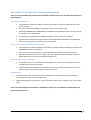
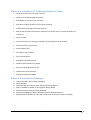
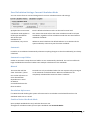
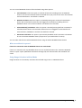
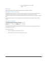
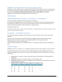
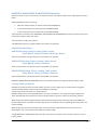
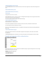
The two values to look up and the two columns to look up are specified as arrays using curly brackets. You should NOT enter this formula as an array formula. Often it is better to reference ranges that contain the values rather than use arrays. This example assumes that J34:K34 contains “superphone” and ”defense”, and J33:K33 contains “Product” and “Sector”. AVLOOKUP2(J34:K34,A1:E7,”Users”,”Asc”,”None”,J33:K33) = 5 Multicolumnlookupwithcolumnsthatarenotadjacent
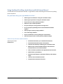
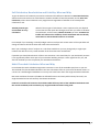
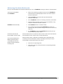
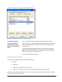
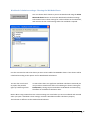
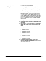
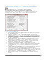
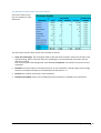
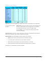
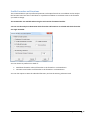
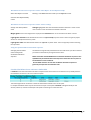
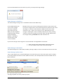
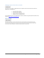
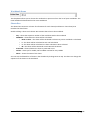
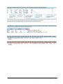
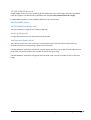
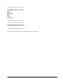
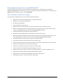
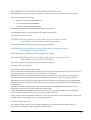
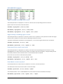
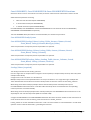
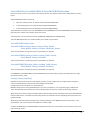
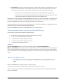
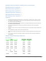
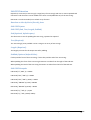
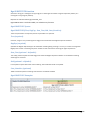
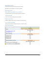
When the columns that you want to lookup are not next to one another you can use the COL.ARRAY function to create an array that makes the data adjacent. So if you want to look up the spend for a Sector and Channel the function would look like this: AVLOOKUP2(COL.ARRAY(C45,A45),A1:E7,”Spend”,”Asc”,”None”,{“Sector”,”Channel”}) UsingRanges,6‐cellarrayformulainD44:E46
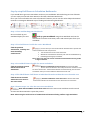
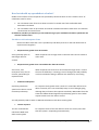
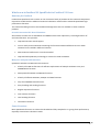
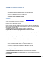
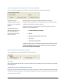
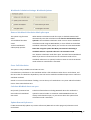
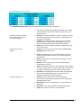
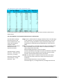
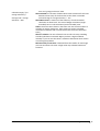
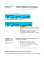
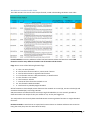
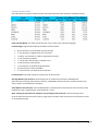
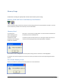
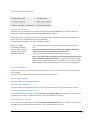
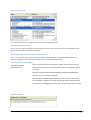
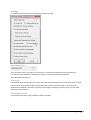
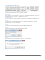
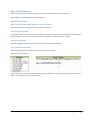
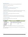
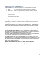
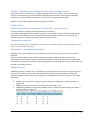
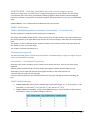
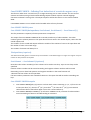
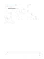
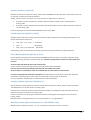
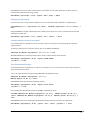
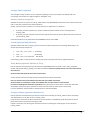
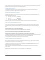
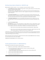
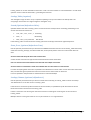
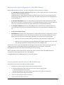
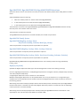
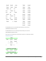
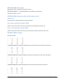
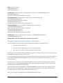
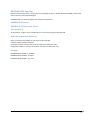
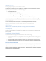
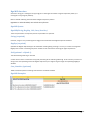
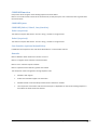
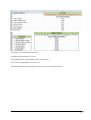
This is an example of using AVLOOKUP2 as a multi‐cell array formula. The formula is entered into D44:E46 as an array formula using Ctrl‐Shift‐Enter, and returns six results because there are three rows to lookup (44:46, each row has 3 columns to lookup) and two columns (D:E) to return from. The example looks up “direct” “superphone” and “defense” in the columns labelled “Channel” “product” and “sector” and returns the values from the corresponding row in columns “Spend” and “Users” (150 and 5). It then looks up “direct” “superphone” and “mfg” and returns the values 1200 and 80, and finally looks up “retail” “spacecalls” and “mfg” to return the error values “none” and “none”. {AVLOOKUP2(A44:C46,A1:E7,D43:E43,"Not","none",A43:C43)}
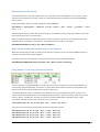
This multi‐cell array formula is the equivalent of these six individual formulas: AVLOOKUP2(A44:C44,A1:E7,D43,"Not","none",A43:C43)
AVLOOKUP2(A44:C44,A1:E7,E43,"Not","none",A43:C43)
AVLOOKUP2(A45:C45,A1:E7,D43,"Not","none",A43:C43)
AVLOOKUP2(A45:C45,A1:E7,E43,"Not","none",A43:C43)
FastExcel V3 User Guide
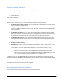
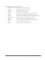
SpeedTools Lookups: Lookup Functions 230