1
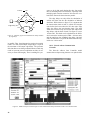
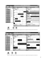
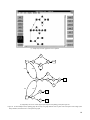
Figure 46. Imposing control edge B
D delays node D behind node B. Since nodes
B and D belong to different iterations, control edge imposes inter-iteration dependency
requiring initial tokens (one, in this example). Design Tool automatically calculates
appropriate number of initial tokens. . . . . . . . . . . . . . . . . . . . . . . . . . . . . . . . . . . . . . . . . . . . . . . . . . 36
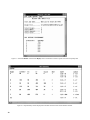
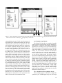
Figure 47. Dataflow graph attributes and timing are displayed in Graph Summary window.
Edge added between nodes B and D requires initial token (OF = 1). . . . . . . . . . . . . . . . . . . . . . . . . . 37
Figure 48. Algorithm function example. . . . . . . . . . . . . . . . . . . . . . . . . . . . . . . . . . . . . . . . . . . . . . . . . 37
Figure 49. Inter-iteration control edges may be initialized with tokens, depending on iteration
number separation. . . . . . . . . . . . . . . . . . . . . . . . . . . . . . . . . . . . . . . . . . . . . . . . . . . . . . . . . . . . . . . . 38
Figure 50. Operating Point plane for three-processor design. . . . . . . . . . . . . . . . . . . . . . . . . . . . . . . . . 39
Figure 51. Updating dataflow graph with design attributes. . . . . . . . . . . . . . . . . . . . . . . . . . . . . . . . . . 39
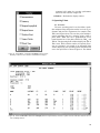
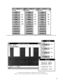
Figure 52. Select View command from File menu in main window to view graph file.
Updated graph for three-processor design is shown. Note added control edges in
middle window.. . . . . . . . . . . . . . . . . . . . . . . . . . . . . . . . . . . . . . . . . . . . . . . . . . . . . . . . . . . . . . . . . . 40
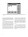
Figure 53. After dataflow graph has been updated, current design may be overwritten.
Alternate design is shown with same number of processors: TBO increases to 350 time
units and TBIO decreases to 590 time units. Subscript alb denotes absolute lower bound.. . . . . . . . 41
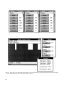
Figure 54. Design Tool warns user when updating a dataflow graph for same number of
processors will overwrite a previous design. . . . . . . . . . . . . . . . . . . . . . . . . . . . . . . . . . . . . . . . . . . . 41
Figure 55. Dataflow graph with communication delays modeled by edge delays. . . . . . . . . . . . . . . . . 42
Figure 56. Dataflow analysis of DFG of figure 55 with communication delays and
Network with Com Controller model.. . . . . . . . . . . . . . . . . . . . . . . . . . . . . . . . . . . . . . . . . . . . . . . . . 42
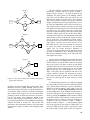
Figure 57. Effect of edge delays on node slack time. Intra-iteration slack of node C is
reduced by C
F edge delay of 20 time units. Inter-iteration slack of node E is reduced
by E
D edge delay of 10 time units. . . . . . . . . . . . . . . . . . . . . . . . . . . . . . . . . . . . . . . . . . . . . . . . . 43
Figure 58. Dataflow analysis of DFG of figure 55 with communication delays and
Network without Com Controller model. . . . . . . . . . . . . . . . . . . . . . . . . . . . . . . . . . . . . . . . . . . . . . . 44
Figure 59. Three graph examples used in demonstrating multiple graph analysis and design. . . . . . . . 45
Figure 60. Capture of multiple graphs with ATAMM graph-entry tool. . . . . . . . . . . . . . . . . . . . . . . . . 46
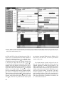
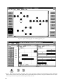
Figure 61. When more than one graph is in graph file, each is given its own Metrics
window and associated displays windows. Minimizing Metrics windows (Graphs 2
and 3 in this figure) hides all opened window displays pertaining to the graphs.
Dataflow analysis of Graph 1 shows four processors are required for an iteration period
of 200 time units.. . . . . . . . . . . . . . . . . . . . . . . . . . . . . . . . . . . . . . . . . . . . . . . . . . . . . . . . . . . . . . . . . 46
Figure 62. Dataflow analysis of Graph 2 shows eight processors are required for
iteration period of 108 time units. . . . . . . . . . . . . . . . . . . . . . . . . . . . . . . . . . . . . . . . . . . . . . . . . . . . . 47
Figure 63. Dataflow analysis of Graph 3 shows four processors are required for
iteration period of 134 time units. . . . . . . . . . . . . . . . . . . . . . . . . . . . . . . . . . . . . . . . . . . . . . . . . . . . . 47
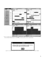
Figure 64. Parallel Graph Execution window summarizes processor requirements for
all graphs intended to execute in parallel. Since it is assumed that phasing between graphs
cannot be controlled in parallel graph strategy, total processor requirement is worst case, or
sum of individual processor requirements. . . . . . . . . . . . . . . . . . . . . . . . . . . . . . . . . . . . . . . . . . . . . . 48
Figure 65. Time multiplex strategy assumes phasing between graphs can be controlled by
defining a finite delay between inputs to graphs. . . . . . . . . . . . . . . . . . . . . . . . . . . . . . . . . . . . . . . . . 49
vii