1
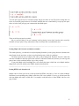
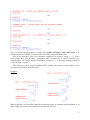
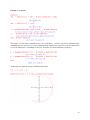
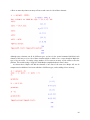
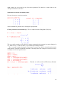
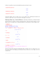
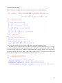
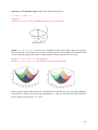
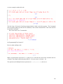
numeric, symbolic, or graphic! We see an example of a symbolic spreadsheet, which is an Excel style
sheet filled with perhaps a table of integrals, as you might find in a book of integrals! Spiffy!
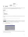
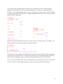
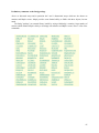
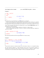
When you have a living command going, right-click to see list of options and suggestions, this is the
context menu. Ie, it depends where you are as to what you see listed on this menu. I don't get the context
items as they describe, but later we shall see why.
A paragraph means a word-processor type of text paragraph, but fancy equation display is built in.
Perhaps this is a better place to write a math paper than in Word with Equation 3.0, we shall see. This is
the end of Topic 2.
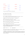
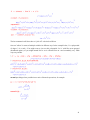
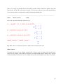
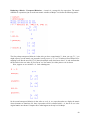
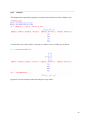
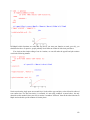
Topic 3 is on numeric computations. The operator % is called the ditto operator, and causes the
previous result to be placed as input to a subsequent operation. First examples are with integer math. For
floating point, they point out that integers are maintained until the very end. Use evalf() to get a floating
point number from something. Another evaluator called value() does something different, not quite sure
of the difference yet. Value seems to get a more perfect symbolic result, rather than a FP result. An
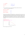
example is the sum of an infinite series which might include PI. You say evalf(%, 50) to get a result to
50 decimal places. We have now seen how to enter series, product and summations.
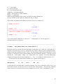
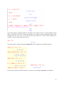
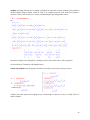
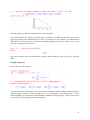
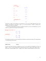
You say convert(%,polar) to convert a complex number like 5+4*I to polar. Note that cap I is the
imaginary I, and you must show multiplication with the *.
The expo "e" is represented as exp(1.0), but pi is Pi, the Gamma function is GAMMA.
My right-click mechanism is definitely not working!!! The end of this topic 3 confirms that notion
that has been accumulating!
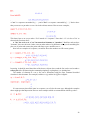
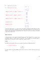
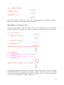
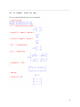
Topic 4 is algebraic computations. You create an expression using the := operator (what language
was that, I forget: Algol? ). Then later you can process that expression. expand() does just what you
expect, and factor(%) does the reverse. Function simplify() uses trig identities to declutter a messy
expression, such as sin^2 + cos^2 would become just 1. Function normal() removes common factors
from a num/den expression. The operator := is the assignment operator, assigning an expression to some
variable name you make up. You maybe define A, and then later say eval(A,x=1); Notice that semicolon
seems to end any command (again, some language is the basis here, need some history soon). The eval
function puts variables to selected values, the result is in general still symbolic, as opposed to evalf.
Conversion is a large world. You can convert to sum of partial fractions (parfrac).
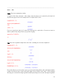
Here is how you define a symbolic function: f := x – x^2+1/2. Then you can put anything you want in
later for x, such as f(2) or f(a+b). The strangely named function unapply does the same thing.
Next, we used assignment to define an object that is an equation: equation := 2*x+1 = x. Then later
you can use solve(equation,{x}) to get all the roots, notice the funny brackets here. You can also
evaluate both sides of an equation using eval(equation, x=2), the sides will be the same if you picked a
root.
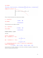
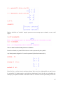
Next, we can solve systems of equations, very nice indeed. Trig and abs values are allowed. Holy
cow! It also does a system of inequalities.
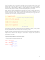
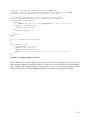
Topic 5 is about graphics. We see that the term with(plot) brings in a class of C++ routines which
you can then use, perhaps this is standard C++ terminology, I forget. So we bring in plots and plottools.
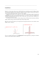
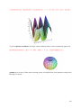
The opening example is a stunning simple animation, that consumes a lot of my CPU. Next is an
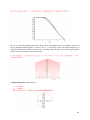
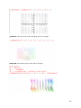
inequality system visualization plot.
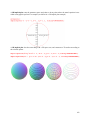
OK, very impressive, and this is where you need a modern day PC and not some old 486 that would
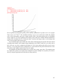
slug along on these rotations. 2D and 3D plots, change lighting (not shown), rotate, etc.
131