1
Chapter 3: Tutorial
7
subbofit -M 0 < testdata1.txt
and you should obtain something like
9.569862e-01 9.104554e-01 5.291858e-02 1.617363e+00
In this particular case, the method of moments provides better estimates than the ones
obtained via maximum-likelihood. Of course the associated log-likelihood is smaller. In order
to obtain more details on the procedure of fitting you can use the option ‘-V’. For more details
Chapter 5 [Fitting Subbotin Density], page 10.
Another interesting feature is the possibility of fitting just the b and a parameters, providing
the “true” value of m directly from the command line. This is useful when you work with
normalized data whose mean has been previously subtracted. Since this is a quite common
situation subbofit provides the ‘-m’ command line option. With the file generated above do
subbofit -m 0 < testdata1.txt
and you should obtain
8.808684e-01 8.777596e-01 0.000000e+00 1.616923e+00
and in this case the variation in the fitted parameters is relatively low.
3.2 Graphic Tutorial
Now let’s start gnuplot and see how the programs in SUBBOTOOLS can be used inside its
graphic environment. Simply type
gnuplot
and you will be greeted by a fairly large amount of informations and, finally, a prompt. As a
first exercise let’s compare the result of our fitting procedure with the original function. Using
gnuplot>set log y
gnuplot>plot "<subbofit -O 2 < testdata.txt" title "fit",\
>exp(-abs(x))/2 title "th."
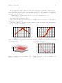
you can produce a graph similar to the one in Fig.1
The option ‘-O 2’ print for each point of the file ‘testdata1.txt’ the value of the probability
density associated with the fitted parameters. gnuplot interprets this output and produces the
corresponding graph. With our small sample the obtained estimate is notably different from the
theoretical Laplace density from which the data were originally generated.
A similar comparison can be performed on the distribution function using the command
gnuplot>set key top left
gnuplot>unset log y
gnuplot>plot "<subbofit -O 1 < testdata1.txt’’ title "fit",\
>(x<0?exp(-abs(x))/2:1.-exp(-abs(x))/2) title "th."
where the option ‘-O 1’ now prints the value of the estimated distribution function for each
input points. The result you should obtain is similar to the one reported in Fig.2.
The program subboshow is conceived for the visual exploration the Subbotin “reduced” loklikelihood. For a precise definition Chapter 5 [Fitting Subbotin Density], page 10. The program
takes a set of observations and print out the associated value of the Subbotin reduced negative
log-likelihood for a grid of b and m values. Using the previously generated observations, try the
following
gnuplot>splot "< subboshow -b0.5:1.5 -m-.1:.11 <testdata.txt ",\
> i 0 notitle w l
and you will obtain a 3D plot representing the negative log-likelihood of the dataset similar
to Fig. 3 .